
Fingerprinting audio recording locations with machine learning
While taking an Audio Signal Processing course at UVic, I came across the Norris-Eyring and Sabine formulas to estimate reverberation time. Some of the criteria for estimating reverberation time required the volume of a room. I started to wonder if this criteria could be reversed to estimate the volume of a room, and built my final project around this idea. The report is presented below. It's quite outdated (2016) at this point and only exists as a historical artifact. However, if it interests you to know more, don't hesitate to reach out! I'd be happy to share the code and data.
Abstract
This report describes an experiment in machine learning and reverb analysis. The experiment attempts to distinguish if a music file is dry (studio) or wet with a reverb (concert). A music collection of 100 songs in the hip hop genre were used and split into two sets. The first set was a simple .au to .wav conversion and the other set had a convolutional reverb applied to it, to sound as if it was recorded in a concert. The MFCC’s of the audio files were extracted and used to create a dataset to feed into a Linear Support Vector Machine algorithm and a Neural Network.
1 Introduction
1.1 Motivation
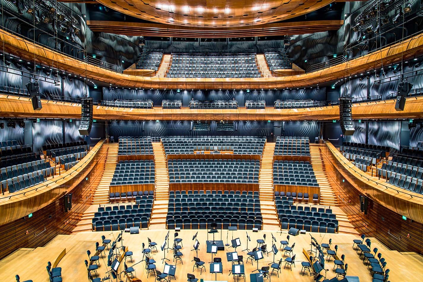
Music is defined by more than just the notes that compose a song. If a song is played in a small room, it will sound vastly different than if played in a big room. If a violin is played, the makeup of the strings, the body style, and material it was built with will play a large part in how it sounds. The way sound bounces off of its surroundings explains the previous examples, and is called reverb.
In the modern world, musicians often lean on synthetic sounds to recreate different soundscapes. To sound natural, it could be preferable to start with a real instrument baseline before adding any further audio processing. If music is defined by more than just the notes that compose a song, it becomes apparent that this is not a trivial task.
Take the violin example. To isolate the violin strings from the body and the room, you could remove the reverb caused by the room, followed by removing the reverb caused by the body. You could approach the problem in two ways. The first is to know the exact dimensions and material composition of the room, walls, floor ceiling, and violin body and perform a de-convolution with this information. This method might sound unnatural. The second approach is to record a room impulse response of the environment, and of the violin body and then use de-convolution to isolate the strings.
However, this experiment seeks to determine if it might be possible to listen to an audio file, and directly extract information about its environment. The approaches of establishing the environment dimensions/composition or creating a RIR could be bypassed entirely in the pursuit of isolation.
1.2 Reverberation
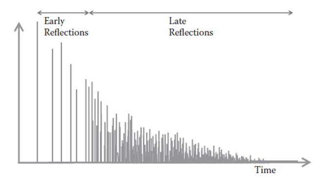
When a sound source emits audio in an environment, there is a direct path from the speaker to the listener. However, there are also other paths that the sound takes to reach the listener, by bouncing off of walls, or objects. These paths take a longer time, and carry a delay with them as well. This is reverberation. There are early reflections and late reflections. Early reflections are related to the parameters of the environment, while late reflections appear more randomly and more frequently. (Reiss & McPherson, 2015)1
1.2.1 Convolutional Reverb
Convolutional reverb works by taking the convolving an audio file with an impulse response of an environment. The best method is by using a sine impulse. The output will sound as if your original audio file was recorded in the same environment as the impulse. (Reiss & McPherson, 2015)1
1.2.2 Algorithmic Reverb
Algorithmic reverb uses infinite impulse response filters (all-pass and comb) to produce a gradually decaying series of reflections. (Reiss & McPherson, 2015)1 These generally don’t sound as convincing as convolutional reverb.
2 Preliminary Decisions
In machine learning there are many paths to apply it. Mature libraries of algorithms exist on most platforms, with python being a strong MATLAB contender.
2.1 Software Environment
MATLAB was chosen due to the familiarity of the language and many inbuilt tools for machine learning. While large libraries exist for C++ and Python, they don’t have the same quality documentation and examples as MATLAB.
2.2 Machine Learning Algorithms
Linear SVM and Neural Networks will be examined in this report. While there are many other options out there, these two are simple to implement in MATLAB.
2.3 GUI Options
MATLAB has an App Designer application with high quality documentation. This will be used for GUI prototyping. App Designer replaces their old GUI maker “GUIDE,” and was chosen over it because of continued support.
3 Convolutional Reverb and Audio Processing
3.1 Dataset
The dataset “GTZAN Genre Collection” was used for the well-known paper in genre classification "Musical genre classification of audio signals" by G. Tzanetakis and P. Cook. The dataset consists of 1000 audio tracks each 30 seconds long. It contains 10 genres, each represented by 100 tracks. The tracks are all 22050Hz Mono 16-bit audio files converted into .wav format. (Tzanetakis)2
Using only 1 channel of audio at 22050Hz reduces the amount of information significantly, but also allows for faster computations on the data and helps with managing the data. The genre hiphop was selected for no particular reason. Each genre contained 100 sound files.
3.2 RIR – Room Impulse Responses
When a source records sound inside of a room, the reverberation is characterized by the room impulse response. Typically, a quick and short sound like a starting pistol or a hand clap is made in the room. The best method is by using a sine impulse. Once an RIR is available, it can be convolved with an input audio signal. This makes the audio file sound as if it was recorded in the same room as the RIR. There are many free sources online for room impulse responses.
This experiment used two different room impulse responses, acquired from Samplicity (Roos, 2016)3 and Voxengo (Vaneev, 2016)4.
- Concert Hall
- Small Room
The RIR were down sampled to 22050 hz upon import to match the audio file sampling rate.
3.3 Audio Files
The audio files files were converted from .au file format to .wav and labled as dry. A read_audio.m script was created with a switch to allow the user to convert the audio into a wav file as either a dry output or convolved with an RIR by calling the func_oa_fft.m function (described below). For this project, 90 files of the hip hop genre were converted into wav as 270 output files for dry, concert and small room conditions. 10 remained untouched for classroom demonstration purposes.
3.4 Convolutional Reverb Function
The function func_oa_fft.m reads an input audio file and an input RIR file. It then performs an overlap-add linear convolution to produce a reverbed output file. The following figure shows how the algorithm works and the pseudocode from which func_oa_fft.m was derived from. (Paolo, 2016)5
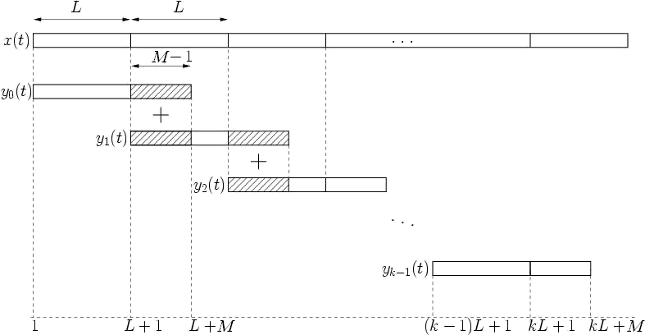
Algorithm 1 (OA for linear convolution)
Evaluate the best value of N and L(L>0, N = M+L-1 nearest to pwr of 2).

Nx = length(x);
H = FFT(h,N) (zero-padded FFT)
i = 1
y = zeros(1, M+Nx-1)
while i <= Nx (Nx: the last index of x[n])
        il = min(i+L-1,Nx)
        yt = IFFT( FFT(x(i:il),N) \* H, N)
        k = min(i+N-1,M+Nx-1)
        y(i:k) = y(i:k) + yt(1:k-i+1) (add the overlapped output blocks)
        i = i+L
end
Figure 3 - Pseudocode of Overlap-add Convolution Method from https://en.wikipedia.org/wiki/Overlap%E2%80%93add_method
3.5 Batch Processing Reverb Outputs
The read_audio.m script is capable of batch processing a folder full of audio. A for loop was used to convolve these files one by one with a room impulse response or to simply convert to wav format.
Each output was stored as dry_filename.wav, smallroom_filename.wav, concert_filename.wav. This format was used for clarity in the data feature extraction step (See section 4.1).
Despite running through 270 songs, the processing of each reverb was almost trivial. Noticeably, Concert Hall took the longest time to process.
| Room Impulse Response | Time to Process (s) |
|---|---|
| Dry | 4.105889 seconds |
| Small Room | 10.738989 seconds |
| Concert Hall | 11.964029 seconds |
4 Environment Extraction with Machine Learning
MATLAB has numerous inbuilt machine learning algorithms that can be used. The Statistics and Machine Learning Toolbox has a great app for the purpose named ‘Classification Learner.’
Please see Appendix A for more details.
4.1 Data Feature Extraction
The original execution involved training the model with audio files as a raw input stream of data. However, upon attempt, it was apparent that the data sets produced by each audio file would be too computationally expensive. In music analysis literature, a set of features called the Mel-Frequency Cepstral Coefficients (MFCC) are the standard input for determining audio and speech characteristics. MFCC analysis is based on the assumption that the human ear acts as a filter that concentrates only on certain frequency components. (Kishore, 2003)6.
Two hundred and seventy wav files were imported into matlab for classification purposes. The script inputNN.m was used to import and create a data set with the following steps:
- Retrieve a list of all files stored in a directory. Directory consists of 90 dry samples, 90 small room samples, 90 concert hall samples.
- To reduce computation time, the audio file was truncated to obtain only the first 15 seconds of music.
- Compute the MFCCs of each audio file with HTK MFCC MATLAB version 1.2 (Wojcicki, 2011)7. Each MFCC computation produced 13 attributes, with 28 samples per song.
- Store the successive attributes and samples into an input matrix
INPUT1. - Determine by file name if the audio being imported is dry, small room, or concert hall, assign numeric value of 1, 2, 3 respectively. (See Section 3.5)
- Store the successive descriptions into a response matrix
RESPONSE1.
From there, two matrices were created. One is the input attribute matrix, and the other is the target matrix. For the classification learner app (See Appendix A), the input format dictates that the response matrix be concatenated with the input matrix. For Neural Networks, the input and target matrixes are kept separate. On this machine, the process took 10 minutes. This is quite an expensive process even on an i7 quad core CPU with 16 GB of ram and further optimization needs to be considered.
The result was a 13 attribute input matrix with 7644 samples (NN_input.mat) and a response matrix with 7644 mappings to dry, small room, or concert (NN_target.mat).
A 14x7644 matrix (NN_data.mat) was also created for compact storage purposes and for MATLAB’s classification learner app.
4.2 Dry vs Concert Hall Results
For this section, a subset of 5096 samples (omitting small room) were fed into the trainers as either dry or concert hall. The accuracy of measurement was very reasonable for both the Linear SVM and Neural Network classifiers.
4.2.1 Linear SVM
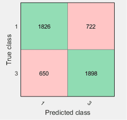
The Linear SVM produced an accuracy of 73.1%. The confusion matrix is presented below.
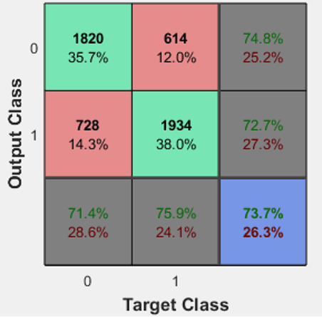
4.2.2 Neural Network
The Neural Network produced an accuracy of 73.7%. The confusion matrix and network diagram is presented below.
4.3 Summary of Findings
A 3 class attempt was also done with 7644 samples that were fed into the trainers as dry, small room or concert hall. The accuracy of measurement diminished by about 10%. This is likely due to the fact that the data set is not large enough to accurately classify the small room samples. [Confusion Matrix omitted]
The following table lays out a summary of the findings. Both methods produced similar results.
| Model | 2 Class Accuracy | 3 Class Accuracy |
|---|---|---|
| Linear SVM | 73.1% | 62.9% |
| Neural Network | 73.7% | 63.4% |
5 Summary and Application
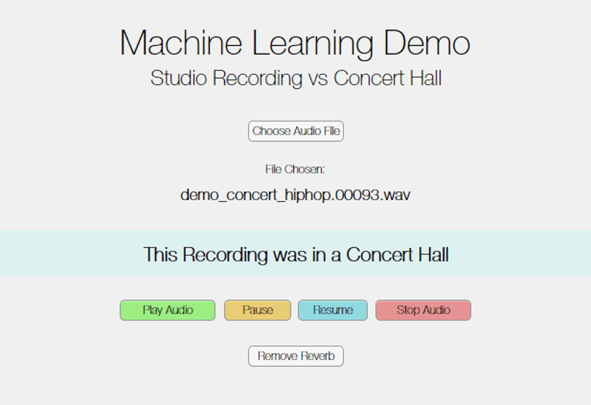
The 2 class Linear Vector Machine model was used to create a proof of concept application.
5.1 Proof of Concept Application
An application was created with MATLAB’s App Designer. The user selects an audio file to determine what environment (“Studio” or “Concert Hall”) it was recorded in. An audio player object is created that lets the user play, pause or stop the sound. If the recording was determined to be in a concert hall, the user can choose to get rid of the concert environment to hear how the audio might have sounded like in a studio.
5.2 Limitations
The Linear SVM model in the application is trained on the MFCC features of 90 audio files that are truncated to 15 seconds and have a sampling rate of 22050Hz and just 1 channel. This provided 5096 total samples for the model to train on.
A good machine learning data set should contain hundreds of thousands to millions of samples to become viable. For this experiment, the choice to reduce the sample pool and the amount of audio information was made to reduce the speed of computations and improve the management of the data.
The model was trained using the hip hop genre of music, and has only been tested on that genre.
The environments for wet samples are simulated with a convolutional reverb that was created specifically for this experiment. Therefore, if the wet output files have any artifacts from the convolutional reverb algorithm implemented, then the model could mistake those artifacts as what we are trying to define as wet audio. Therefore, the results might differ from other implementations of convolutional reverb to produce wet samples.
The machine learning demo application can import any audio file. However, the current model will only meaningfully interpret a subset of audio that it was trained to recognize. The criteria for audio files is presented below.
| Criteria | Description |
|---|---|
| Format | .wav |
| Sampling | 22050Hz |
| BitRate | 176kbps |
| Channels | Mono |
| Genre | Hip Hop |
5.3 Future Work
Future work could potentially turn this into a viable environment analysis solution.
- MFCCs were chosen as the features of the music as they are standard in audio analysis. Other options should be identified for reverb evaluation purposes.
- The model was trained on a small subset of data. The amount of samples in future tests should increase to have as many samples as possible. Hundreds of thousands to a million samples should be obtained.
- Audio input files should be higher quality, and incorporate the full stereo signal into the data set.
- The wet reference samples should be from a variety of sources to eliminate any artifacts or signatures that may be present in a specific convolutional reverb application.
- Create a much better de-convolution function.
6 Appendix A - Machine Learning in MATLAB
A MathWorks Webinar provides a great tutorial to get familiar with the machine learning tools. This section walks through some general examples of machine learning and its application. (Gupta, 2014)8.
The dataset used was BANK. It was the result of a direct marketing campaign with phone calls. It contains 45,210 observations with 16 attributes of a client, and 1 column of responses consisting of yes or no (S. Moro, Cortez, & Rita, 2014).
6.1 Supervised and Unsupervised Learning
There are two main scenarios of machine learning.
6.1.1 Supervised Learning
Supervised learning’s goal is to make predictions based on a set of observations. This method is “supervised” because it requires the data set to have both attributes and responses to those attributes.
- Classification – The data is used to predict a category. This is the type of machine learning implemented in this report. We provide attributes in the form of music files and seek to classify them by room type.
- Regression – The data is used to predict a value. Common examples are determining the value of a house for sale by comparing it to the houses sold in the area.
- Anomaly Detection – The data is used to define what normal behavior looks like, and identify anything that might be strange. For example, if you take numerous normal credit card transaction data points then the anomaly might be a fraudulent credit card transaction (Rohrer, 2016).
6.1.2 Unsupervised Learning
There might not be any responses, or classification of data points in the dataset. Then, the problem becomes one of determining if there is any order that exists in the data points. This is useful for taking large amounts of complex data and determining if there is any grouping in the data points. (Rohrer, 2016)9
6.2 Data Preperation
A 10% subset of the data was imported from a semicolon delimited csv file consisting of 4521 observations, 16 attributes and 1 response into a table. Attribute variable names were extracted from the first row of the table and stored into a cell array named ‘name’.
% Import from file
bank = func_import('bank.csv',';');
% Extract top row headings
names = bank.Properties.VariableNames;

% Convert all the categorical variables into nominal arrays
[nrows, ncols] = size(bank);
category = false(1,ncols);
for i = 1:ncols
    if isa(bank.(names{i}),'cell') || isa(bank.(names{i}),'nominal')
        category(i) = true;
        bank.(names{i}) = nominal(bank.(names{i}));
    end
end

% Logical array keeping track of categorical attributes
catPred = category(1:end-1);
The data was segregated into a response array Y consisting of the last column and predictor matrix X consisting of N-1 columns.
% Response
Y = bank.y;

% Predictor matrix
X = bank(:,1:end-1);
6.3 Cross Validation
Cross Validation is used to test the results of a model. The techniques can be as simple as splitting the data in half or more complicated methods, such as k-fold and leave-one-out validation. K-fold is an interesting method, as it divides the data up into k sets and trains k times, treating different sets as a holdout set each time. This enables every observation to be used for both training and testing. (McLachlan, Do, & Ambroise, 2004)10.
This exercise chose the simpler route, by splitting the original dataset into two subsets. One subset is for training purposes and the other is for testing purposes. For this example, cvpartition was used to split the dataset into 60% for training purposes (Xtrain, Ytrain) and held 40% for testing purposes (Xtest, Ytest).
% 40% of the data will be held for testing purposes
cv = cvpartition(height(bank),'holdout',0.40);

% Training set
Xtrain = X(training(cv),:);
Ytrain = Y(training(cv),:);
% Test set
Xtest = X(test(cv),:);
Ytest = Y(test(cv),:);
7 References
Footnotes
-
Reiss, J. D., & McPherson, A. P. (2015). Audio Effects: Theory, Implementation, and Application. CRC Press. ↩ ↩2 ↩3
-
Tzanetakis, G. (n.d.). Marsyas. Retrieved from GTZAN Genre Collection: http://marsyas.info/downloads/datasets.html ↩
-
Roos, E. P. (2016). Samplicity. Retrieved from Samplicity’s Bricasti M7 Impulse Response Library v1.1: http://www.samplicity.com/bricasti-m7-impulse-responses/ ↩
-
Vaneev, A. (2016). Free Reverb Impulse Responses. Retrieved from Voxengo: http://www.voxengo.com/impulses/ ↩
-
Paolo, S. (2016, June 4). Wikipedia. Retrieved from Overlap-add Method: https://en.wikipedia.org/wiki/Overlap%E2%80%93add_method ↩
-
Kishore, P. (2003). Spectrogram, Cepstrum and Mel-Frequency Analysis. Retrieved from Speech Technology: A Practical Introduction : http://www.speech.cs.cmu.edu/15-492/slides/03_mfcc.pdf ↩
-
Wojcicki, K. (2011, Sept 19). HTK MFCC MATLAB ver 1.2. Retrieved from MATLAB File Exchange: https://www.mathworks.com/matlabcentral/fileexchange/32849-htk-mfcc-matlab ↩
-
Gupta, A. (2014, July 30). Mathworks Matlab File Exchange. Retrieved from Machine Learning with MATLAB: https://www.mathworks.com/matlabcentral/fileexchange/42744-machine-learning-with-matlab/content/Machine%20Learning/Classification/html/MachineLearning.html ↩
-
Rohrer, B. (2016, April 4). How to choose algorithms for Microsoft Azure Machine Learning. Retrieved from Microsoft Azue: https://azure.microsoft.com/en-us/documentation/articles/machine-learning-algorithm-choice/ ↩
-
McLachlan, G. J., Do, K.-A., & Ambroise, C. (2004). Analyzing microarray gene expression data. Wiley. ↩